Motivation
We wanted to challenge our machine learning abilities with a challenge that could have a huge impact on the world. Diabetes is a disease known for being undiagnosed for years when people have it. Since Diabetes affects 400 million people in the world, the goal of this project was to use machine learning to determine the most effective way of detecting whether or not an individual has diabetes or not.
According to the CDC, Diabetes is a chronic (long-lasting) health condition that affects how your body turns food into energy. The human body naturally breaks down the food you eat into a sugar called glucose, and releases the glucose into your bloodstream. Then the pancreas releases insulin which allows your cells to receive the glucose in your bloodstream. However, people with diabetes either cannot produce insulin or the insulin being created does not work. This leaves too high of blood sugar levels in their bloodstream which can later cause heart disease, vision loss, and kidney disease.
Dataset
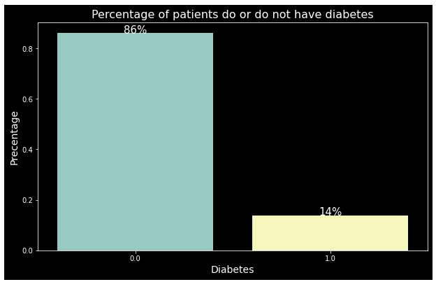
The dataset used for this project was found on Kaggle.com. The survey was performed via telephone and was conducted by the CDC in 2015 that asked participants numerous health related questions. The original survey resulted in 330 features in total with 253,680 responses. The modified dataset found on Kaggle is a reduced version with only 21 features and contains only two classes for the target variable: 0 for no diabetes, and 1 for pre-diabetes or diabetes. It is important to note that the dataset is not balanced.
The features that are included in the modified dataset are as follows: high blood pressure, high cholesterol, cholesterol check[ed], BMI, smoker, stroke, heart disease or attack, physical activity, fruits, vegetables, consumes heavy alcohol, any healthcare, afford doctor’s visit, general health, physical health, mental health, difficulty walking, sex, age, education, and income. The 21 features were chosen because of their potential relevance to detecting diabetes in an individual, and range from health conditions to lifestyle choices and factors.
Observations
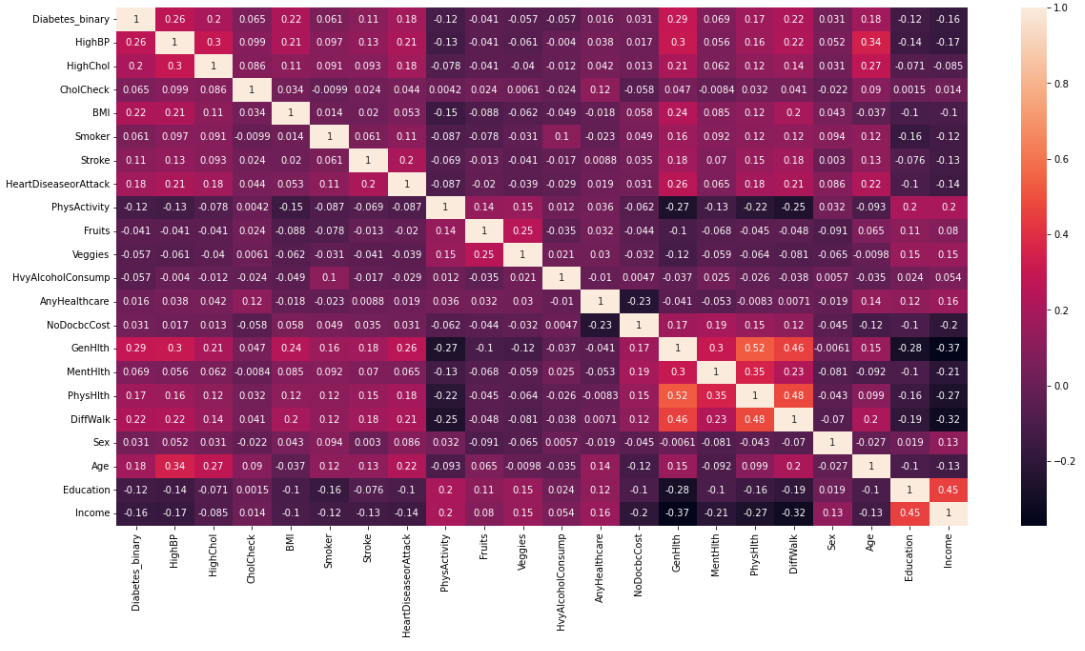
In our initial observation, we found that high blood pressure, high cholesterol, BMI, heart disease [or] attack, general health, and age all have significant correlation with the target variable. In addition, there is a slightly noticeable negative correlation with physical activity, education, and income with the outcome variable, meaning that diabetes is less prominent in individuals where these features are higher.
Machine Learning Algorithms
When it comes to creating a model for a binary classification problem, such as this one, there are many suitable and popular algorithms. We chose to use k-Nearest Neighbors (KNN), Logistic Regression, and Neural Network to create a diabetes classifier, all which are very different, because we wanted to see how they would compare to one another in performance and accuracy.
Experiment
K-Nearest Neighbors (KNN)
KNN is a simple, but very powerful supervised classification algorithm that classifies based on a similarity measure. KNN utilizes “lazy” learning because the model does not actually learn anything. Instead, when a new data is introduced, we find its k-nearest neighbor from the training data. This makes it very important to have a balanced and consistent training data.
To make our diabetes predictions with the KNN model, a new data is compared with the entire training data and takes the output of its nearest neighbor (in this case, the mode). The nearest neighbor is measured by Euclidean distance. The formula for Euclidean distance is defined as: $$dist = \sqrt{\Sigma_{n=1}^\infty (a_k-b_k)^2}$$ , where p is the number of features and 𝑎𝑘 and 𝑏𝑘 are, respectively, the kth feature of a and b.
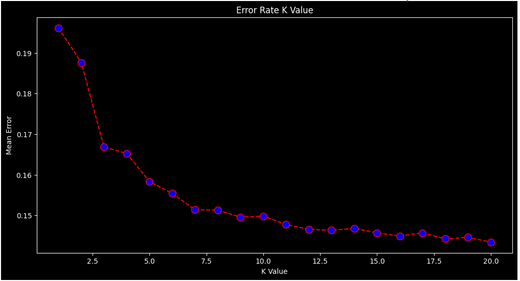
Choosing the most optimal k is important to achieve maximum accuracy. We found that when k is less than or equal to 10, it leads to unstable decision boundaries, and for k greater than 10, the decision boundaries were smoother. For our KNN algorithm, we tested every k from 1 to 20. The optimal parameter for k would be where the error rate is at its lowest. Shown in graph below, the most optimal parameter was between 16 to 20. Due to our problem being a binary classification problem, 17, an odd k value, was chosen.

Logistic Regression
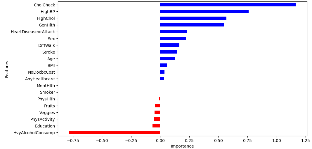
Logistic Regression is another supervised machine learning algorithm we used to determine the probability of an individual having diabetes. We wanted to determine the correlation of each feature with the target variable and see how they could affect the model. In the initial interpretation of the correlation coefficient of each feature, we can see that CholCheck, HighBP, GenHlth, and HighChol have significant influence on the model, whereas features like MentHlth and Smoker have little to no significance on the model.
The model uses a logistic function to model the conditional probability of the label Y (pre-diabetic or diabetic) variables X (the 21 features). The continuous result is then mapped to a closed set [0, 1] using a sigmoid function, which is used to further interpret probability. In order to classify the continuous value, we rounded the probability to 0 or 1 to make a prediction. $$P=(Y|X)$$
Artificial Neural Network
In our artificial neural network (ANN), we use deep learning to perform binary classification on our dataset. This algorithm is completely different from our Logistic Model because it uses a backward propagation of errors with respect to the neural network's weights.
In our initial experimentation, we use a simple ANN architecture: one input layer of 20 nodes, two hidden layers of 8 nodes each that use the Rectified Linear Unit (ReLu) activation function, and one output layer of 1 node that uses Sigmoid activation function. The ReLu activation function outputs the input directly if it is positive and zero otherwise to effectively help the model learn faster, while the Sigmoid function reduces the output to a value from 0.0 to 1.0 representing a probability.
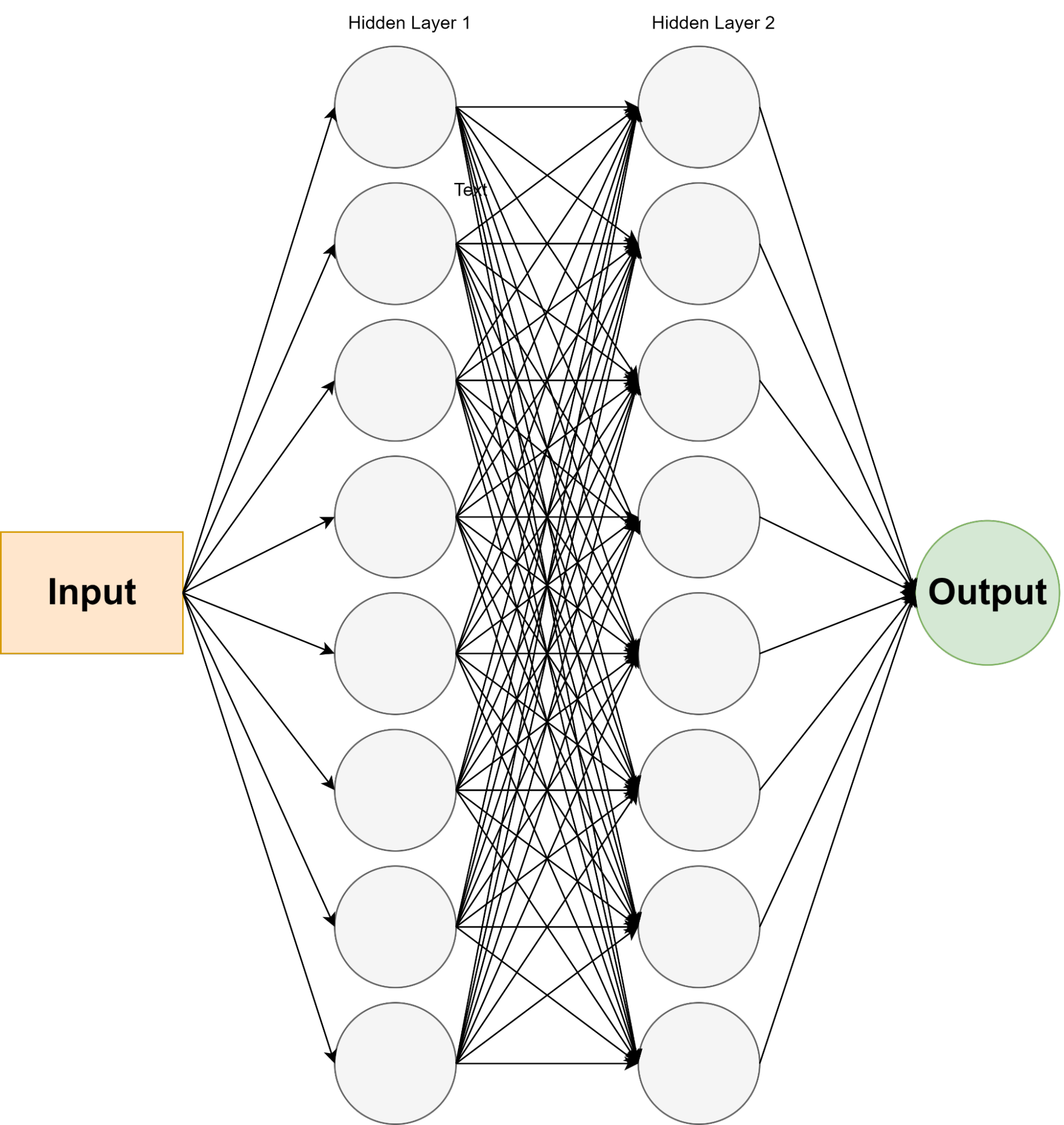
To optimize our ANN, we used a grid test algorithm of various hyperparameter to find the optimal parameters for the neural network. We experimented with different optimizers, loss functions, learning rates, batch sizes, number of nodes, and epochs which resulted in the most optimal hyperparameter: Adam optimizer with the default learning rate, Binary Cross Entropy loss function, the default batch size, 8 nodes for each hidden layer, and a total of 100 epochs.
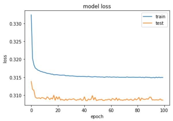
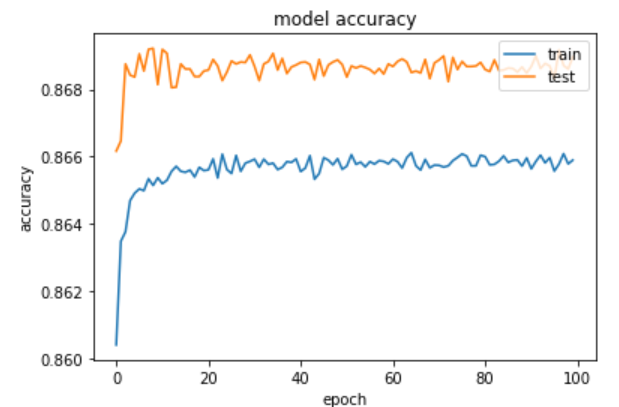
We plotted the accuracy and loss to epochs to see how the model was improving each iteration. The elbow-shaped graph for the training data in the model loss plot shows that maximum accuracy was achieved, which corresponds with the model accuracy plot.
Results
ROC Curve
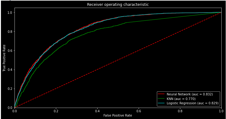
The ROC curve represents the discrimination between the classes that the models made. Having an ROC curve that is significantly different from a straight line shows that the classifier model is not making random guesses. Looking at the ROC curve from all of our models we can clearly see that our models were not making random guesses, and were using the training data to make inferences about the testing data. The area under the curve (AUC) shows how well the classifier is able to distinguish between the different classes. Looking at each models AUC, we can see that the Neural Network and Logistic Regression models were able to distinguish between the positive and negative classes much more than the KNN algorithm.
Based on a rough classifying system, AUC can be interpreted as follows: 90 -100 = excellent; 80 - 90 = good; 70 - 80 = fair; 60 - 70 = poor; 50 - 60 = fail
Conclusion
Through the experiment we have found that Logistic Regression was the best technique to use for binary classification. It was more effective than KNN should in the ROC/AUC and the F1 score. Since Neural Network has very similar scores in the Confusion Matrix, Classification Report, and AUC, we chose to compare the time it took to run each technique. We found that it was more efficient to use Logistic Regression in comparison to Neural Network. In the end, we found that Logistic Regression is the best technique between these three when it comes to binary classification.
Obstacles
One issue we faced was from the beginning of our experiment, when we didn’t look at what our dataset consisted of. We first looked at the features and the number of samples, but we didn’t consider the imbalance in the dataset. Near the end when the team was looking at the uneven F1 score from the classification report, we felt that there was something wrong. We searched up why the uneven F1 score would happen and found that an imbalanced dataset would do that. Looking at the percentage from each class, 14% of the samples has diabetes and the other 86% did not have diabetes.
To fix the imbalance dataset, we added class weights to Logistic Regression. Logistic Regression was chosen over KNN due to its higher precision and was chosen over Neural Network due to the time that it took to find the optimal parameters. The confusion matrix and F1 score seemed to match the dataset more and shown below. Although the class weights didn’t give the optimal F1 score, it was much more evenly distributed and the accuracy seemed to match our model much better. Had we done this again, we could have added custom class weights to further optimize the model.
References
Teboul, A., Centers for Disease Control and Prevention (2011). Diabetes Health Indicators Dataset.
